使用lasso在高维模型中进行推断

Using the lasso for inference in high-dimensional models
9 September 2019David Drukker, Executive Director of Econometrics and Di Liu, Senior Econometrician

Why use lasso to do inference about coefficients in high-dimensional models?

High-dimensional models, which have too many potential covariates for the sample size at hand, are increasingly common in applied research. The lasso, discussed in the previous post, can be used to estimate the coefficients of interest in a high-dimensional model. This post discusses commands in Stata 16 that estimate the coefficients of interest in a high-dimensional model.

An example helps us discuss the issues at hand. We have an extract of the data Sunyer et al. (2017) used to estimate the effect of air pollution on the response time of primary school children. The model is

We want to estimate the effect of no2_class on htime and to estimate a confidence interval for the size of this effect. The problem is that there are 252 controls in  x , but we have only 1,084 observations. The usual method of regressing htime on no2_class and all the controls in  x  will not produce reliable estimates for  γ  when we include all 252 controls.

Looking a little more closely at our problem, we see that many of the controls are second-order terms. We think that we need to include some of these terms, but not too many, along with no2_class to get a good approximation to the process that generated the data.

In technical terms, our model is an example of a sparse high-dimensional model. The model is high-dimensional in that the number of controls in  x  that could potentially be included is too large to reliably estimate  γ  when all of them are included in the regression. The model is sparse in that the number of controls that actually need to be included is small, relative to the sample size.

Returning to our example, let’s define  x ~  to be the subset of  x  that must be included to get a good estimate of  γ  for the sample size. If we knew  x ~ , we could use the model

The sparse structure implies that we could estimate  γ  by regressing htime on no2_class and  x ~ , if we knew  x ~ . But we don’t know which of the 252 potential controls in  x  belong in  x ~ . So we have a covariate-selection problem, and we have to solve it to estimate  γ .

The lasso discussed in the last post, immediately offers two possible solutions. First, it seems that we could use the lasso estimates of the coefficients. This does not work because the penalty term in the lasso biases its coefficient estimates toward zero. The lack of standard errors for the lasso estimates also prevents this approach from working. Second, it seems that using the covariates selected by the lasso would allow us to estimate  γ . Some versions of this second option work, but some explanation is required.

One approach that suggests itself is the following simple postselection (SPS) estimator. The SPS estimator is a multistep estimator. First, the SPS estimator uses a lasso of the dependent variable on the covariates of interest and the control covariates to select which control covariates should be included. (The covariates of interest are not penalized so that they are always included in the model.) Second, it regresses the dependent variable on the covariates of interest and the control covariates included in the lasso run in the first step.

The SPS estimator produces unreliable inference for  γ . Leeb and Pötscher (2008) showed that estimators like the SPS that include the control covariates selected by the lasso in a subsequent regression produce unreliable inference. Formally, Leeb and Pötscher (2008) showed that estimators like the SPS estimator generally do not have a large-sample normal distribution and that using the usual large-sample theory can produce unreliable inference in finite samples.

The root of the problem is that the lasso cannot always find the covariates with small coefficients. An example of a small coefficient is one whose magnitude is not zero but is less than twice its standard error. (The technical definition includes a broader range but is harder to explain.) In repeated samples, the lasso sometimes includes covariates with small coefficients, and it sometimes excludes these covariates. The sample-to-sample variation of which covariates are included and the intermittent omitted-variable bias caused by missing some relevant covariates prevent the large-sample distribution of the SPS estimator from being normal. This lack of normality is not just a theoretical issue. Many simulations have shown that the inference produced by estimators like the SPS is unreliable in finite samples; see, for example, Belloni, Chernozhukov, and Hansen (2014) and Belloni, Chernozhukov, and Wei (2016).

Belloni et al. (2012), Belloni, Chernozhukov, and Hansen (2014), Belloni, Chernozhukov, and Wei (2016), and Chernozhukov et al. (2018) derived three types of estimators that provide reliable inference for  γ  after using covariate selection to determine which covariates belong in  x ~ . These types are known as partialing-out (PO) estimators, double-selection (DS) estimators, and cross-fit partialing-out (XPO) estimators. Figure 1 details the commands in Stata 16 that implement these types of estimators for several different models.

Figure 1. Stata 16 commands

A PO estimator

In the remainder of this post, we discuss some examples using a linear model and provide some intuition behind the three types of estimators. We discuss a PO estimator first, and we begin our discussion of a PO estimator with an example.

We use breathe7.dta, which is an extract of the data used by Sunyer et al. (2017), in our examples. We use local macros to store the list of control covariates. In the output below, we put the list of continuous controls in the local macro ccontrols, and we put the list factor-variable controls in the local macro fcontrols. We then use Stata’s factor-variable notation to put all the potential controls in the local macro ctrls. ctrls contains the continuous controls, the indicators from the factor controls, and the interactions between the continuous controls and the indicators created from the factor controls.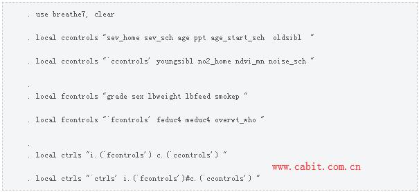

The c., i., and # notations are Stata’s way of specifying whether variables are continuous or categorical (factor) and whether they are interacted. c.(`ccontrols’) specifies that each variable in the local macro ccontrols enter the list of potential controls as a continuous variable. i.(`fcontrols’) specifies that each variable in the local macro fcontrols enter the list of the potential controls as a set of indicators for each level for the variable. i.(`fcontrols’)#c.(`ccontrols’) specifies that interactions of each level of each factor variable in the local macro fcontrols be interacted with each continuous variable in the local macro ccontrols.

We now describe the outcome variable htime, the covariate of interest (no2_class), the continuous controls, and the factor-variable controls. The potential controls in the model will include the continuous controls, the factor controls, and interactions between the continuous and the factor controls.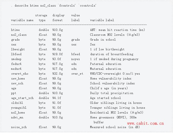

Now, we use the linear partialing-out estimator implemented in poregress to estimate the effect of no2_class on htime. The option controls() specifies potential control covariates. In this example, we included the levels of the factor controls, the levels of the continuous controls, and the interactions between the factor controls and the continuous controls. We used estimates store to store these results in memory under the name poplug.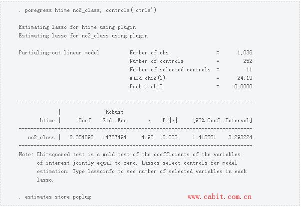

For the moment, let’s focus on the estimate and its interpretation. The results imply that another microgram of NO2 per cubic meter increases the mean reaction time by 2.35 milliseconds.

Only the coefficient on the covariate of interest is estimated. The coefficients on the control covariates are not estimated. The cost of using covariate-selection methods is that these estimators do not produce estimates for the coefficients on the control covariates.

The PO estimators extend the standard partialing-out estimator of obtaining some regression coefficients after removing the effects of other covariates. See section 3-2f in Wooldridge (2020) for an introduction to the standard method. The PO estimators use multiple lassos to select the control covariates whose impacts should be removed from the dependent variable and from the covariates of interest. A regression of the partialed-out dependent variable on the partialed-out covariates of interest estimates the coefficients of interest.

The mechanics of the PO estimators provide some context for some more advanced comments on this approach. For simplicity, we consider a linear model for the outcome  y  with one covariate of interest ( d ) and the potential controls  x .

Here are the steps involved in a PO estimator for  γ  in (1).

1. Use a lasso of  y  on  x  to select covariates  x ~ y  that predict  y .
2. Regress  y  on  x ~ y , and let  y ~  be residuals from this regression.
3. Use a lasso of  d  on  x  to select covariates  x ~ d  that predict  d .
4. Regress  d  on  x ~ d , and let  d ~  be residuals from this regression.
5. Regress  y ~  on  d ~  to get estimate and standard error for  γ .

Heuristically, the moment conditions used in step 5 are unrelated to the selected covariates. Formally, the moments conditions used in step 5 have been orthogonalized, or “immunized”, to small mistakes in covariate selection. This robustness to the mistakes that the lasso makes in covariate selection is why the estimator provides a reliable estimate of  γ . See Chernozhukov, Hansen, and Spindler (2015a,b) for formal discussions.

Now that we are familiar with the PO approach, let’s take another look at the output.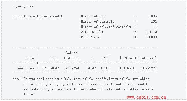

The output indicates that the estimator used a plug-in-based lasso for htime and a plug-in-based lasso for no2_class to select the controls. The plug-in is the default method for selecting the lasso penalty parameter. We discuss the tradeoffs of using other methods below in the section Selecting the lasso penalty parameter.

We also see that only 11 of the 252 potential controls were selected as controls by these lassos. We can use lassocoef to find out which controls were included in each lasso.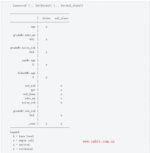

We see that age and four interaction terms were included in the lasso for htime. We also see that sev_sch, ppt, no2_home, ndvi_mn, noise_sch, and an interaction term were included in the lasso for no2_class. Some of the variables used in interaction terms were included in both lassos, but otherwise the sets of included controls are distinct.

We could have used lassoknots instead of lassocoef to find out which controls were included in each lasso, which we illustrate in the output below.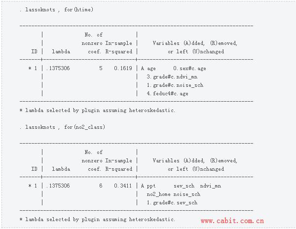

A DS estimator

The DS estimators extend the PO approach. In short, the DS estimators include the extra control covariates that make the estimator robust to the mistakes that the lasso makes in selecting covariates that affect the outcome.

To be more concrete, we use the linear DS estimator implemented in dsregress to estimate the effect of no2_class on htime. We use the option controls() to specify the same set of potential control covariates as we did for poregress. We store the results in memory under the name dsplug.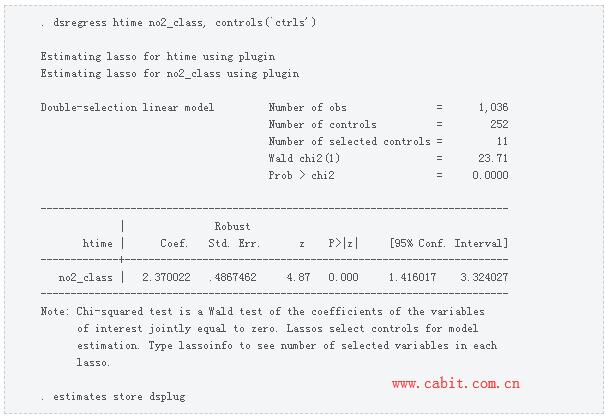

The interpretation is the same as for poregress, and the point estimate is almost the same.

The mechanics of the DS estimators also provide some context for some more advanced comments on this approach. Here are steps for the DS for the linear model in (1).

1. Use a lasso of  y  on  x  to select covariates  x ~ y  that predict  y .
2. Use a lasso of  d  on  x  to select covariates  x ~ d  that predict  d .
3. Let  x ~ u  be the union of the covariates in  x ~ y  and  x ~ d .
4. Regress  y  on  d  and  x ~ u .
   The estimation results for the coefficient on  d  are the estimation results for  γ .

The DS estimator has two chances to find the relevant controls. Belloni, Chernozhukov, and Wei (2016) report that the DS estimator performed a little better than the PO in their simulations, although the two estimators have the same large-sample properties. The better finite-sample performance of the DS estimator might be due to it including a control found in either lasso in a single regression instead of using the selected controls in separate regressions.

Comparing the DS and PO steps, we see that the PO and the DS estimators use the same lassos to select controls in this model with one covariate of interest.

As with poregress, we could use lassocoef or lassoknots to see which controls were selected in each of the lassos. We omit these examples because they produce the same results as for the example using poregress above.

An XPO estimator

Cross-fitting, which is also known as double machine learning (DML), is a split-sample estimation technique that Chernozhukov et al. (2018) derived to create versions of PO estimators that have better theoretical properties and provide better finite sample performance. The most important theoretical difference is that the XPO estimators require a weaker sparsity condition than the single-sample PO estimators. In practice, this means that XPO estimators can provide reliable inference about processes that include more controls than single-sample PO estimators can handle.

The XPO estimators have better properties because the split-sample techniques further reduce the impact of covariate selection on the estimator for  γ .

It’s the combination of a sample-splitting technique with a PO estimator that gives XPO estimators their reliability. Chernozhukov et al. (2018) show that just using a split-sample estimation technique is not sufficient to make an inferential estimator that uses the lasso or another machine-learning method that uses covariate-selection robust to covariate selection mistakes.

We now use the linear XPO estimator implemented in xporegress to estimate the effect of no2_class on htime.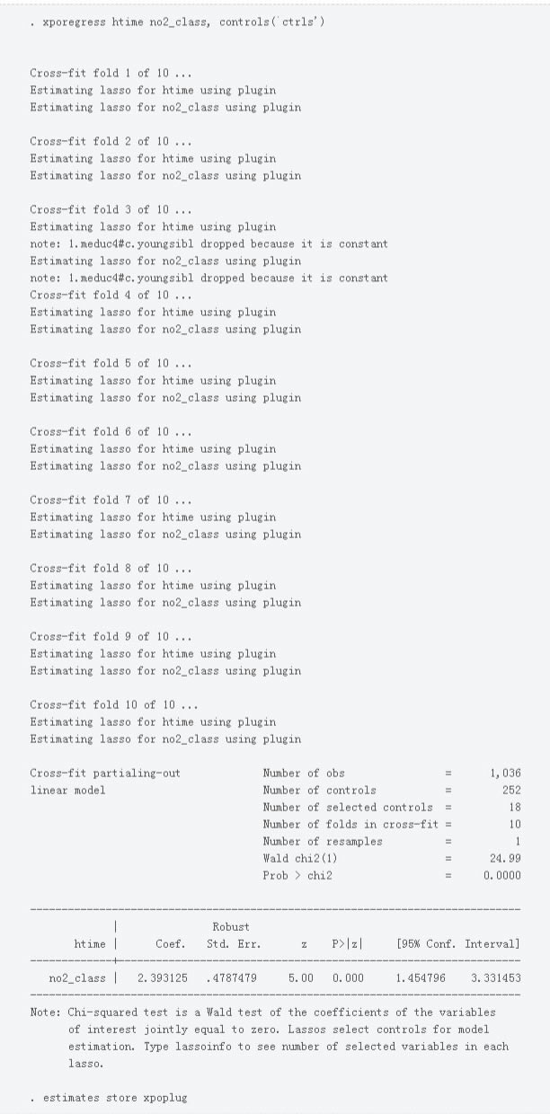

The interpretation is the same as for the previous estimators, and the point estimate is similar.

The output shows that a part of the process was repeated over 10 folds.
Split-sample techniques divide the data into subsets called “folds”.
To clarify what is being done, let’s consider the steps that would be
performed by a linear XPO estimator for the  γ  in (1) when there are only 2 folds in the model.

1. Split data into 2 folds called A and B.
2. Use the data in fold A to select the covariates and to estimate the postselection coefficients.
   1. Use a lasso of  y  on  x  to select the controls  x ~ y  that predict  y .
   2. Regress  y  on  x ~ y , and let  β ~ A  be the estimated coefficients.
   3. Use a lasso of  d  on  x  to select the controls  x ~ d  that predict  d .
   4. Regress  d  on  x ~ d , and let  δ ~ A  be the estimated coefficients.
3. Fill in the residuals for  y  and for  d  in fold B using the coefficients estimated using the data in fold A. Using the data in fold B, do the following:
   1. Fill in the residuals for  y ~ =y −x ~ y β ~ A .
   2. Fill in the residuals for  d ~ =d −x ~ d δ ~ A .
4. Use the data in fold B to select the controls and to estimate the postselection coefficients. Using the data in fold B, do the following:
   1. Use a lasso of  y  on  x  to select the controls  x ~ y  that predict  y .
   2. Regress  y  on  x ~ y , and let  β ~ B  be the estimated coefficients.
   3. Use a lasso of  d  on  x  to select the controls  x ~ d  that predict  d .
   4. Regress  d  on  x ~ d , and let  δ ~ B  be the estimated coefficients.
5. Fill in the residuals in fold A using the coefficients estimated using the data in fold B. Using the data in fold A, do the following:
   1. Fill in the residuals for  y ~ =y −x ~ y β ~ B .
   2. Fill in the residuals for  d ~ =d −x ~ d δ ~ B .
      
6. Now that the residuals are filled in for the whole sample, regress  y ~  on  d ~  to estimate  γ .

When there are 10 folds instead of 2, the algorithm has the same structure. The data are divided into 10 folds. For each fold  k , the data in the other folds are used to select the controls and to estimate the postselection coefficients. The postselection coefficients are then used to fill in the residuals for fold  k . With the full sample, regressing the residuals for  y  on the residuals for  d  estimates  γ .

These steps explain the fold-specific output produced by xporegress.

We recommend using xporegress over poregress and dsregress because it has better large-sample properties and has better finite-sample properties. The cost is that xporegress takes longer than poregress and dsregress because of its fold-level computations.

Selecting the lasso penalty parameter

The inferential-lasso commands that implement PO, DS, and XPO estimators use the plug-in method to select the lasso penalty parameter ( λ ) by default. The value of  λ  specifies the importance of the penalty term in the objective function that lasso minimizes. When the lasso penalty parameter is zero, the lasso yields the ordinary least-squares estimates. The lasso includes fewer covariates as  λ  increases.

When the plug-in method is used to select  λ , the PO, DS, and XPO estimators have proven large-sample properties, as discussed by Belloni et al. (2012) and Belloni, Chernozhukov, and Wei (2016). The plug-in method tends to do a good job of finding the important covariates and does an excellent job of not including extra covariates whose coefficients are zero in the model that best approximates the true process.

The inferential-lasso commands allow you to use cross-validation (CV) or the adaptive lasso to select  λ . CV and the adaptive lasso tend to do an excellent job of finding the important covariates, but they tend to include extra covariates whose coefficients are zero in the model that best approximates the true process. Including these extra covariates can affect the reliability of the resulting inference, even though the point estimates do not change by that much.

The CV and the adaptive lasso can be used for sensitivity analysis that investigates whether reasonable changes in  λ  cause large changes in the point estimates. To illustrate, we compare the DS estimates obtained when  λ  is selected by the plug-in method with the DS estimates obtained when  λ  is selected by CV. We also compare the DS plug-in-based estimates with those obtained when  λ  is selected using the adaptive lasso.

In the output below, we quietly estimate the effect using dsregress when using CV and the adaptive lasso to select  λ . First, we use option selection(cv) to make dsregress use CV-based lassos. We use estimates store to store these results in memory under the name dscv. Second, we use option selection(adaptive) to make dsregress use the adaptive lasso for covariate selection. We use estimates store to store these results in memory under the name dsadaptive. We specify option rseed() to make the sample splits used by CV and by the adaptive lasso reproducible.

Now, we use lassoinfo to look at the numbers of covariates selected by each lasso in each of the three versions of dsregress.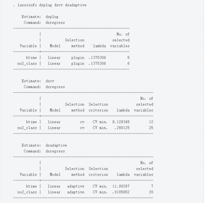

We see that CV selected more covariates than the adaptive lasso and that the adaptive lasso selected more covariates than the the plug-in method. This result is typical.

We now use estimates table to display the point estimates produced by the three versions of the DS estimator.

The point estimates are similar across the different methods for selecting  λ . The sensitivity analysis found no instability in the plug-in-based estimates.

Hand-specified sensitivity analysis

In this section, we illustrate how to use a particular value for  λ  in a sensitivity analysis. We begin by using estimates restore to restore the dscv results that used CV-based lassos in computing the DS estimator.

We now use lassoknots to display the knots table from doing CV in a lasso of no2_class on the potential controls.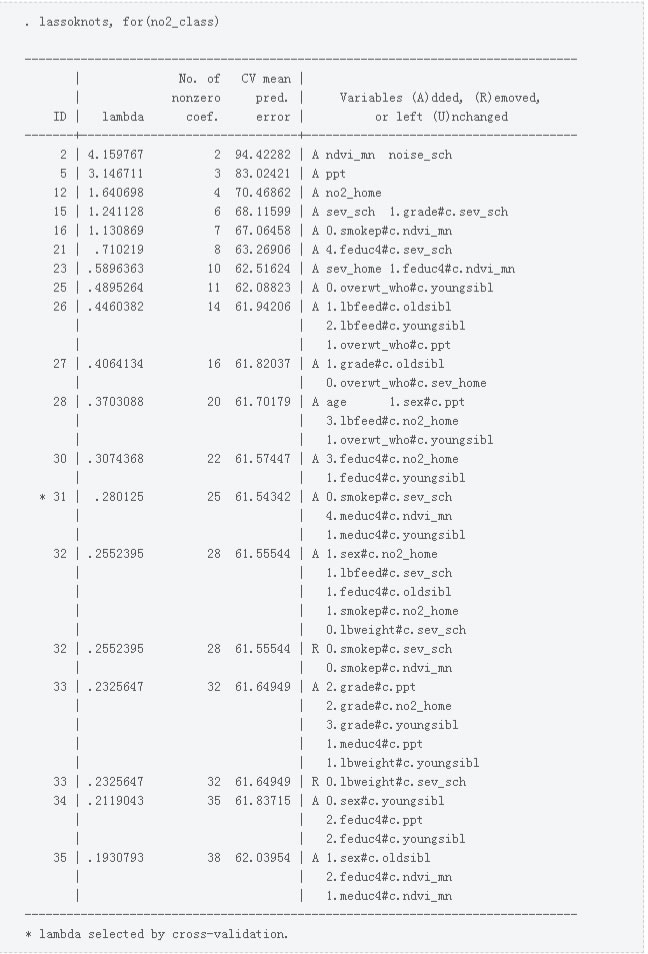

The  λ  selected by CV has ID=31. This  λ  value produced a CV mean prediction error of 61.5, and it caused the lasso to include 25 controls. The  λ  with ID=23 would produce a CV mean prediction error of 62.5, and it would cause the lasso to include only 10 controls.

The  λ  with ID=23 seems like a good candidate for sensitivity analysis. In the output below, we illustrate how to use lassoselect to specify that the  λ  with ID=23 be the selected value for  λ  for the lasso of no2_class on the controls. We also illustrate how to store these results in memory under the name hand.

Now, we use dsregress with option reestimate to estimate  γ  by DS using the hand-specified value for  λ .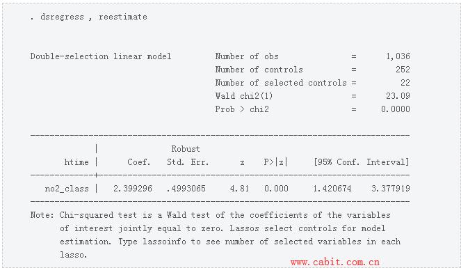

The point estimate for  γ  does not change by much.

Conclusion

This post discussed the problems involved in estimating the coefficients of interest in a high-dimensional model. It also presented several methods implemented in Stata 16 for estimating these coefficients.

This post discussed only estimators for linear models with exogenous covariates. The Stata 16 LASSO manual discusses methods and commands for logit models, Poisson models, and linear models with endogenous covariates of interest.

References

Belloni, A., D. Chen, V. Chernozhukov, and C. Hansen. 2012. Sparse models and methods for optimal instruments with an application to eminent domain. Econometrica 80: 2369–2429.

Belloni, A., V. Chernozhukov, and C. Hansen. 2014. Inference on treatment effects after selection among high-dimensional controls. Review of Economic Studies 81: 608–650.

Belloni, A., V. Chernozhukov, and Y. Wei. 2016. Post-selection inference for generalized linear models with many controls. Journal of Business & Economic Statistics 34: 606–619.

Chernozhukov, V., D. Chetverikov, M. Demirer, E. Duflo, C. Hansen, W. Newey, and J. Robins. 2018. Double/debiased machine learning for treatment and structural parameters. Econometrics Journal 21: C1–C68.

Chernozhukov, V., C. Hansen, and M. Spindler. 2015a. Post-selection and post-regularization inference in linear models with many controls and instruments. American Economic Review 105: 486–90.

——. 2015b. Valid post-selection and post-regularization inference: An elementary, general approach. Annual Review of Economics 7: 649–688.

Leeb, H., and B. M. Pötscher. 2008. Sparse estimators and the oracle property, or the return of Hodges estimator. Journal of Econometrics 142: 201–211.

Sunyer, J., E. Suades-González, R. García-Esteban, I. Rivas, J. Pujol, M. Alvarez-Pedrerol, J. Forns, X. Querol, and X. Basagaña. 2017. Traffic-related air pollution and attention in primary school children: Short-term association. Epidemiology 28: 181–189.

Wooldridge, J. M. 2020. Introductory Econometrics: A Modern Approach. 7th ed. Boston, MA: Cengage-Learning.

相关文档